| Type of paper: | Essay |
| Categories: | Ecology Pollution Air pollution |
| Pages: | 6 |
| Wordcount: | 1588 words |
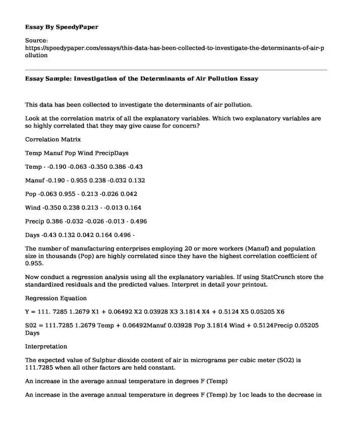
This data has been collected to investigate the determinants of air pollution.

Look at the correlation matrix of all the explanatory variables. Which two explanatory variables are so highly correlated that they may give cause for concern?
Correlation Matrix
Temp Manuf Pop Wind PrecipDays
Temp - -0.190 -0.063 -0.350 0.386 -0.43
Manuf -0.190 - 0.955 0.238 -0.032 0.132
Pop -0.063 0.955 - 0.213 -0.026 0.042
Wind -0.350 0.238 0.213 - -0.013 0.164
Precip 0.386 -0.032 -0.026 -0.013 - 0.496
Days -0.43 0.132 0.042 0.164 0.496 -
The number of manufacturing enterprises employing 20 or more workers (Manuf) and population size in thousands (Pop) are highly correlated since they have the highest correlation coefficient of 0.955.
Now conduct a regression analysis using all the explanatory variables. If using StatCrunch store the standardized residuals and the predicted values. Interpret in detail your printout.
Regression Equation
Y = 111. 7285 1.2679 X1 + 0.06492 X2 0.03928 X3 3.1814 X4 + 0.5124 X5 0.05205 X6
S02 = 111.7285 1.2679 Temp + 0.06492Manuf 0.03928 Pop 3.1814 Wind + 0.5124Precip 0.05205 Days
Interpretation
The expected value of Sulphur dioxide content of air in micrograms per cubic meter (SO2) is 111.7285 when all other factors are held constant.
An increase in the average annual temperature in degrees F (Temp)
An increase in the average annual temperature in degrees F (Temp) by 1oc leads to the decrease in the expected Sulphur dioxide content of air in micrograms per cubic meter (SO2) by 1.2679 when all other factors are held constant Ceteris Paribus.
i.e. SO2 = 1.2679
Temp
iii. Number of manufacturing enterprises employing 20 or more workers (Manuf)
An increase in the number of manufacturing enterprises by 1 additional worker (Manuf) leads to the increase in the expected Sulphur dioxide content of air in micrograms per cubic meter (SO2) by 0.06492 Ceteris Paribus.
i.e. SO2 = 0.06492
Manuf
iv. Population size in thousands (Pop)
An increase in the population size by an additional one thousands leads to the decrease in the expected Sulphur dioxide content of air in micrograms per cubic meter (SO2) by 0.03928 when all other factors are held constant.
i.e. SO2 = - 0.03928
Pop
iv. Average annual wind speed in miles per hour (Wind)
An increase in the average annual wind speed in miles per hour (Wind) by one additional unit leads to the decrease in the expected Sulphur dioxide content of air in micrograms per cubic meter (SO2) by 3.1814 ceteris Paribus.
i.e. SO2 = -3.1814
Wind
v. Average annual precipitation in inches (Precip)
An increase in the Average annual precipitation in inches (Precip) leads to the increase in the expected Sulphur dioxide content of air in micrograms per cubic meter (SO2) by 0.5124 Ceteris Paribas.
i.e. SO2 = 0.5124
Precip
vi. Average number of days with precipitation per year (Days)
An increase in the average number of days with precipitation per year (Days) by one additional day leads to the decrease in the expected Sulphur dioxide content of air in micrograms per cubic meter (SO2) by 1.2679 Ceteris Paribas.
i.e. SO2= - 0.05205
Days
This data has been collected to investigate the determinants of air pollution.
c. Examine the residual plots (or construct a residual plot of the standardized residuals and the predicted values if using StatCrunch). What do the plots indicate?
By plotting a graph of predicted value against the standardized residuals, we obtain the plots that indicate scope of the data by showing the data which are outside the scope (outliers) and those that are inside the scope and hence relevant.
d. Look at the standardized residuals for each city. You will notice from these and your plots that two cities stand out in the model fit as being outliers. Locate these cities and comment.
The cities that are outliers are Philadelphia and Pittsburgh. The have the highest standardized residuals of 2.23 and 3.61 respectively. The fact that they have the highest standardized residuals indicated that that they are outliers.
e. Using the information in the ANOVA table (part b) and the correlation matrix (part a) comment on if any variables should be eliminated from the regression model.
In order to eliminate variables in the regression model, outliers and data having a high correlation coefficient should be eliminated. For the above case Air Pollution in U.S. Cities, data relating to the (Number of manufacturing enterprises employing 20 or more workers (Manuf) and Population size in thousands (Pop) ) has a high correlation of 0.955 and hence one of the variables should be eliminated. In this case, data relating to Manuf should hence be eliminated. The existence of a high correlation between variables makes the regression equation inefficient and unreliable.
Informational data relating to Air Pollution in U.S. Cities contains outliers with Philadelphia and Pittsburgh cities falling outside the range of scope of data. In this case, the city with the highest residuals standardized residual of 3.61 which is Pittsburg should be eliminated. The fact that the informational data has a high standardized residual indicates that it is an outlier and does not fall within the range of data required and hence it should be eliminated since it makes the regression equation as well as the results unreliable.
PART II
IPS TEXTBOOK PROBLEMS 11.31-11.33 DATA SET ATTACHED IN BLACKBOARD
The following three exercises use the HAPPINESS data set. The World Database of Happiness is an online registry of scientific research on the subjective appreciation of life. It is available at worlddatabaseofhappiness.eur.nl and is directed by Dr. Ruut Veenhoven, Erasmus University, Rotterdam. One inventory presents the average happiness score for various nations between 2007 and 2008. This average is based on individual responses from numerous general population surveys to a general life satisfaction (well-being) question. Scores ranged between 0 (dissatisfied) to 10 (satisfied). The NationMaster Web site, www.nationmaster.com, contains a collection of statistics associated with various nations. For this data set, the factors considered are the GINI Index: measures the degree of inequality in the distribution of income (higher score = greater inequality); the degree of corruption in government (higher score = less corruption); average life expectancy; and the degree of democracy (higher score = more political liberties).
11.31 Predicting a nations average happiness score. Consider the five statistics for each nation: LSI, the average life-satisfaction score; GINI, the GINI index; CORRUPT, the degree of corruption in government; LIFE, the average life expectancy; and DEMOCRACY, a measure of civil and political liberties.
(a) Using numerical and graphical summaries, describe the distribution of each variable (Working in the attached Excel Sheet).
(b) Using numerical and graphical summaries, describe the relationship between each pair of variables. CORRELATIONS (Working in the attached Excel Sheet).
11.32 Building a multiple linear regression model. Lets now build a model to predict the life-satisfaction score, LSI
Question 1(a)
Consider a simple linear regression using GINI as the explanatory variable. Run the regression and summarize the results. Be sure to check assumptions.
GINI Explanatory variable (X)
LSI Dependent variable (Y)
Regression Equation:
Y = 7.0238 0.02014X
LSI = 7.0238 0.02014 GINI
Question 1(b)
Now consider a model using GINI and LIFE. Run the multiple regression and summarize the results. Again be sure to check assumptions.
LSI Dependent variable Y
GINI Explanatory variable X1
LIFE Explanatory variable X2
Linear Regression Equation
Y = -3.82567 + 0.028733 X1 +0.12503 X2
LSI = -3.82567 + 0.028733 Gini + 0.12503 Life
Question 1 (c)
Now consider a model using GINI, LIFE, and DEMOCRACY. Run the multiple regression and summarize the results. Again be sure to check assumptions.
LSI Dependent variable Y
GINI Explanatory variable X1
LIFE Explanatory variable X2
DEMOCRACY Explanatory variable X3
Multiple Regression Equation
Y = -3.2524 + 0.028X1 +0.1063 X2 +0.1857 X3
LSI = -3.2524 + 0.028 Gini +0.1063 Life +0.1857 Democracy
Question 1(d)
Now consider a model using all four explanatory variables. Again summarize the results and check assumptions.
Multi-Regression Equation
Y = -2.7201 + 0.0368X1 +0.0905X2 +0.0392 X3 + 0.1855 X4
LSI = 2.7201 + 0.0368 Gini + 0.0905 Life + 0.0392 Democracy + 0.1855 Corruption
11.33 Selecting from among several models. Refer to the results from the previous exercise.
Question 1(a)
Make a table giving the estimated regression coefficients, standard errors, t statistics, and P-values.
Coefficients Standard Errors T-statistics P-values
LSI 2.720 0.866 -3.141 0.003
Gini 0.037 0.009 3.916 0.0002
Life 0.091 0.011 8.080 1.73E-11
Democracy 0.039 0.066 0.5977 0.552
Corruption 0.186 0.050 3.680 0.0005
Question 1 (b)
Describe how the coefficients and P-values change for the four models.
The expected LSI (the average life-satisfaction score) is 111.7285 when all other factors are held constant.
The GINI index.
An increase in the GINI index leads to the increase in the expected The LSI, the average life-satisfaction score by 0.037 ceteris Paribas.
ssi.e. LSI = 0.037
GNI index
Corruption (The degree of corruption in government)
An increase in the corruption leads to the increase in the LSI, the average life-satisfaction score by 0.091 ceteris Paribas.
i.e. LSI = 0.091
Corruption
LIFE, the average life expectancy
An increase in the corruption leads to an increase in the LSI, the average life-satisfaction score by 0.091 ceteris Paribas.
i.e. LSI = 0.039
Corruption
DEMOCRACY, a measure of civil and political liberties
An increase in the democracy as a measure of civil and political liberties leads to the increase in the LSI (the average life-satisfaction score) by 0.86 ceteris Paribas.
i.e. LSI = 0.186
Democracy
Democracy has the highest probability value of 0.552 while Life has the lower probability value. This means that Life as a factor determining the average life-satisfaction score is more significant as compared to Democracy. Also, the standard error of Life is less and hence has low deviations indicating that it is a significant variable. It is evident that from the above data, thethat standard errors increase with every addition of an extra variable determining the average life-satisfaction score.
Question 1(c)
Based on the table of coefficients, suggest another model. Run that model, summarize the results, and compare it with the other ones. Which model would you choose to explain LSI? Explain.
When LSI is run against GINI, Life, Good health and Economy, it given less standard errors as well as the p-values. The t-statistics are also significant. Hence we can conclude that LSI (average life satisfaction score) is a function of Gini, Life, goo...
Cite this page
Essay Sample: Investigation of the Determinants of Air Pollution. (2019, May 14). Retrieved from https://speedypaper.com/essays/this-data-has-been-collected-to-investigate-the-determinants-of-air-pollution
Request Removal
If you are the original author of this essay and no longer wish to have it published on the SpeedyPaper website, please click below to request its removal:
- Essay Example on How the Relationship Affects Healthiness
- Essay Example on Leadership in Organizations
- Free Essay on the Juvenile Court System
- Free Essay on Examples of Biotechnology That Have Made Improvement in My Life
- Free Paper with an Annotated Bibliography Sample about Electric Vehicles
- English Composition Assignment: Victorian and Modernist Literature. Free Essay
- Essay Sample on American Stability in the 20th Century
Popular categories